SIGGRAPH-2025-Advances--STRAND-BASED-HAI

Hello, I'm Sergei Kulikov from MachineGames and this talk is about strand-based hair in Indiana Jones and the Great Circle.

Here is our agenda for the next 40 minutes. First, we will look at what goals and requirements we had when designing strand hair. I will give a brief overview of the system we ended up with and how its components fit together. Next, we will dive deep into three large parts of our system – rasterization, shading, and composition. We will cover algorithms and performance optimizations we did for those systems to be able to run unfortunately we don't have enough time to cover hair simulation and hair path tracing today so we will focus on the parts that I've mentioned before we begin I want to stress that strand hair system was a large collaborative effort throughout the project development and I want to say huge thank you to everyone who contributed to prototyping developing and shipping strand hair our and its software engine team for beautiful engine that serves as a foundation of our work and of course to our wonderful character art team for their invaluable input and great content they have created with the system. I also want to specifically thank Michael Wynn for setting us on the Strandhair path and making the first working implementation of the system and George Luna for his great work on hair simulation. Ok, let's begin. Why did we decide to focus on Strandhair for the game? Indiana Jones and the Great Circle is a first-person game that puts you in the shoes of Indiana Jones and sets you on an epic cinematic adventure around the globe. It's a story-driven game with a heavy focus on the characters. We have a lot of cutscenes, around four hours of them in total. Also, first-person perspective means that the player gets to see the faces of their enemies up close. And with such a game, our characters need to look as good as possible. Another critical point for us was simplifying hair creation workflow for artists. The game has many characters and we want to free our artists to do creative work. We also have several requirements. First, we always had strict 60fps target for responsive and smooth gameplay. That was a clear goal and all systems that we design have to run at 60fps for all our target platforms. The GPU budget for a system was estimated as 2ms for simulation plus rendering on min-spec at worst case scenario which is around a dozen characters on screen with some of them close to camera. Of course, in simpler scenarios we aim for the hair to be faster than that. We want to avoid putting more work on the artists. We do not want to create two separate versions of each hair asset, so the system has to be fast and robust to be used everywhere. In the end, we only had a couple of assets that still use hair cards, mostly on animals. And assuming those two requirements are met, we want to get the best visual quality we can afford. We want physical correctness, but if we can get a lot of performance by deviating from it, we will do that. I want to explain a bit on how hair creation workflow looked for us. When using hair cards, we have to make the hair card atlas first from strands, then achieve the style we want by placing and sculpting the cards. After that, we need to tweak mesh normals, export everything to the engine, and tweak materials there. When iterating, you often need to repeat a few steps, and most of of those steps are very technical and take a lot of time. But when we use strengths directly, we can get rid of two steps in the pipeline. Now we don't have to do anything with mesh normals, and we don't need to create cards. All that we need to do is style the hair splines directly. We use Xgen Interactive Groom for that, but you can also use Houdini or Xgen or whatever tool you want, and tweak hair materials after export. Each iteration is significantly faster. The differences between workflow are large enough so we can't make one hair version automatically form the other. That's why we don't want to do two versions of our hair.

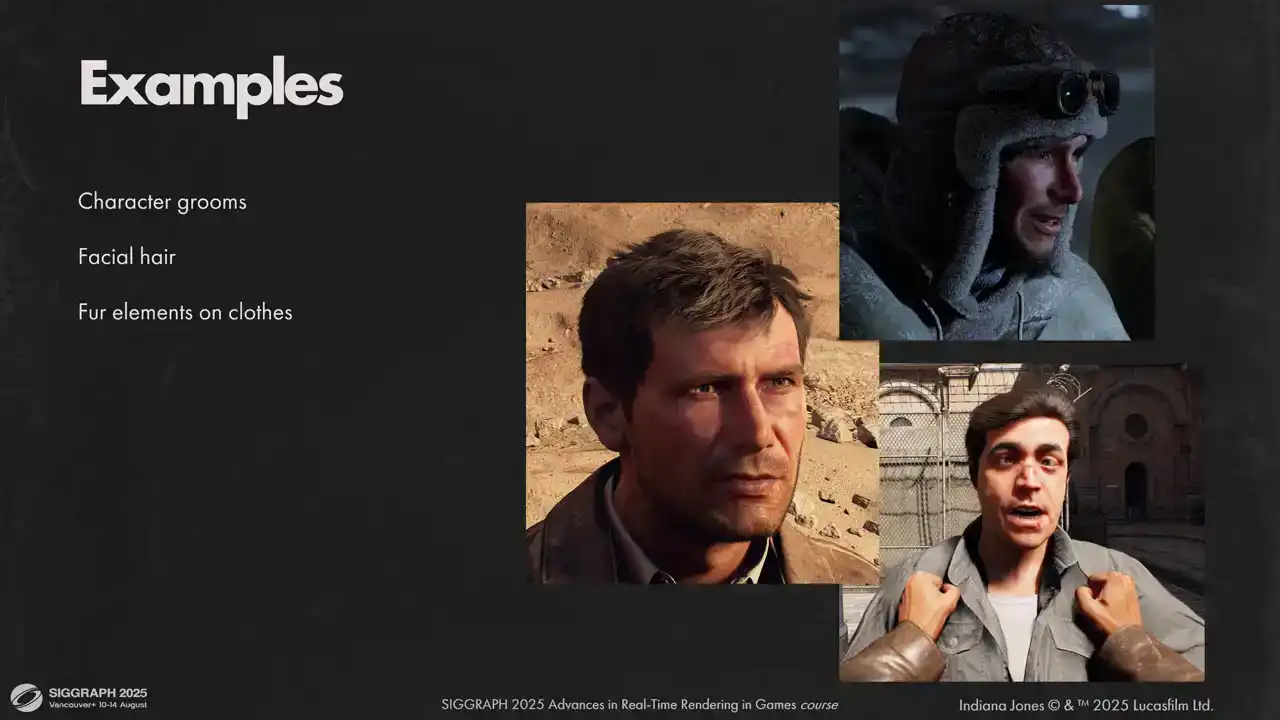
Here are a few examples of what we use the strands for. First, all character grooms and facial hair are done with strands. I think we have about two corpses in the entire game with hair cards. Some fur elements on clothes are also done with strands. For example, this hat and color on Indy's winter jacket. We also tried to use strands for animal fur. It wasn't a complete success, but we ended up using them for some animals, like these spiders and this monkey. Dogs you can see in the game still use hair cards. There were some issues preventing us from using strands on all animals, and we will explore it a bit later. Hair on hands and fingers were kind of last minute additions to the game, but we were quite happy with how it worked out. Before diving into hair pipeline, let me give you a bit of context about the engine Our engine motor is based on it tech 7 and shares a great deal of rendering code with it It uses clustered forward rendering for direct lighting calculations but some opaque passes are deferred, like Diffuse GI. We allocate most of our GPU memory upfront and can't break those limits mid-gameplay. All our shaders are written by graphics engineers from maximum control over the code and maximum performance. The engine also heavily utilizes the sync compute. of our frame is covered by SamadSync work. And here is a general outline of a single rendered frame. Width of each segment does not reflect the actual GPU timings, but rather its place in the frame with regards to work in the neighbor queue. For purposes of this talk, we need to know that we have three large portions of the frame. Common passes such as GPU scene gather, shadows, ray tracing, BVH constructions, and so on. Also lighting passes for opaque pixels and blended geometry rendering. We try to utilize the scene compute by working on blended geometry as early as possible and have some of it finished

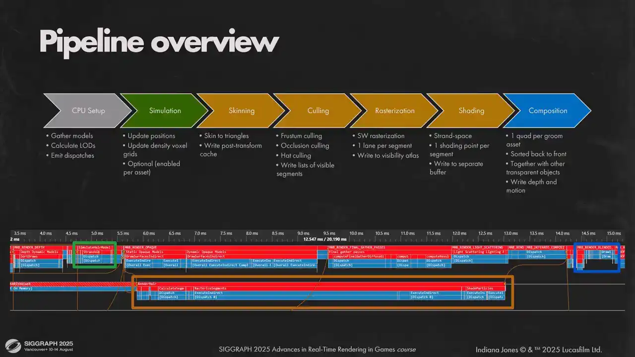
while the main queue draws opaque pixels. Now let's look at our hair rendering pipeline. We have a small CPU setup part that just gathers all hair models in view, calculate appropriate LEDs for them and emits dispatches. On the GPU side side we split the pipeline into three parts. First is simulation. Artists can selected per hair object. We do it on the main graphics cube because we want hair simulation to be done before we start opaque lighting passes. Second part is actually rendering the hair into a layered visibility buffer and doing vertex shading. We do that on a scene compute to overlap calculations with our forward lighting pass and diffuse GI. It allows us to get a more uniform load on the GPU. Hair workloads are very predictable and uniform, so they are filling the gaps in the GPU utilization very nicely. And the last part is to compose rendered here on screen. We treat here as any other transparent geometry in the game and render it back to front in the same path with other geometry. In the lower part of the slide you can see how it fits together with the rest of the frame. And don't be scared about the duration of AsyncCompute passes, the actual workload is much smaller, it just fills the gaps in the graphics queue.

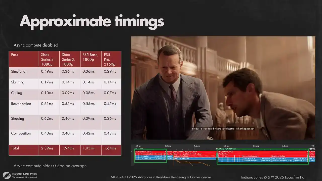
If we disable AsyncCompute, for the average shot we will get the numbers shown on screen. You can see we exceed our budget on Sirius S a little, but when measuring with a sync compute enabled, we get back around half a millisecond, which fits into our predictions. On other hardware, timings for passes are a bit different with respect to each other, but they sum up to pretty much the same numbers.

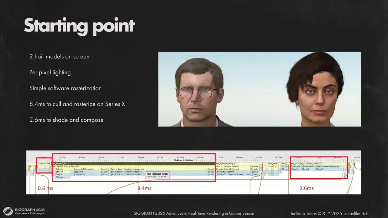
And for perspective, here is one of our first performance measures we did for hair system. Most visual features are already there, except hair shadows on the skin. But as you can see, we had a very long road ahead of us to make it work with our frame budgets.

The first thing we need to do is to find the level of detail for each hair model in view. We don't use separate LOD models, instead we use the common practice of randomizing strand order, and then we can take only a section of that strand buffer, scale thickness of each strand accordingly, and hair shape will still be the same. So the only thing that we need to calculate is a strand number for each model. We do this in three phases. First, on model loading time we limit the maximum number of strands according to quality settings. Small hair models are not reduced because they don't contribute much to rendering time and reduction is much more visible for them.

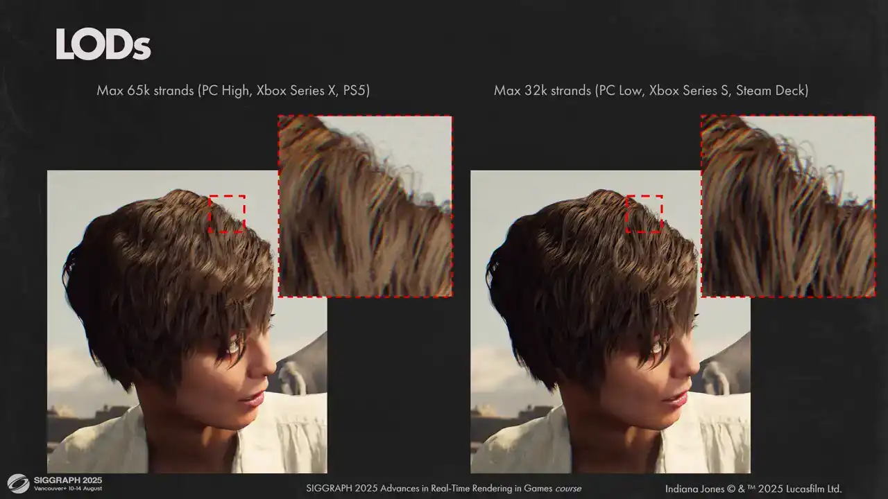
Here you can see two different options for maximum number of strands in the model. On the left is our maximum quality with 65 000 strands and on the right is our minimum quality setting that we use on less powerful hardware. And as you can see, the visual results are close, but lower quality version is darker. This is related to how we do self-shadowing and we will explore that a bit later.

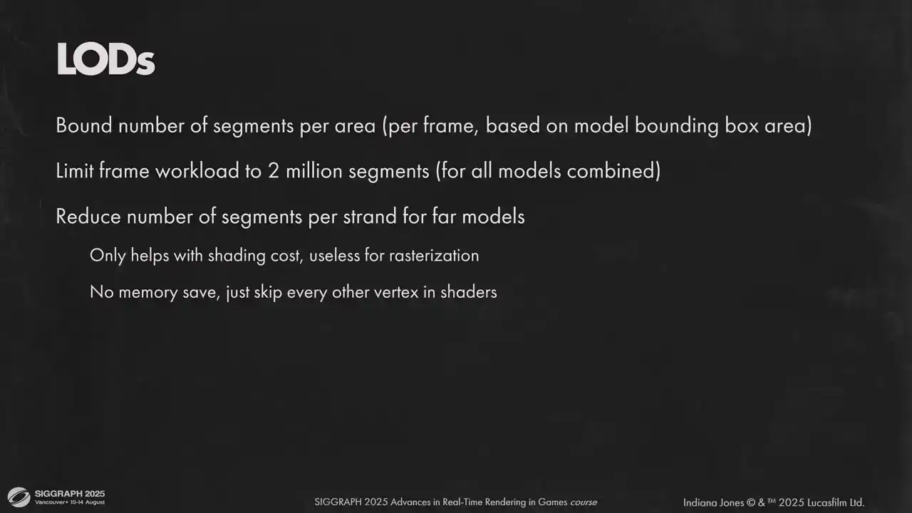
Then, each frame we compute screen area for each hair model and scale its number of strands to maintain a certain limit of rendered segments per visible area. We use an upper boundary of 2000 segments per 64x64 pixel tile on all platforms, as it gives a good visual result and performance for us. Once we have our initial loads calculated for each model, we look at total sediment count for all rendered models and limit it at 2 million segments. If we exceed the limit, we proportionally reduce the number of strands in each model until everything fits into limits. That gives us an upper bound for all per-vertex calculations and for the memory. Additionally, to reduce per-vertex calculations further, we can dynamically skip every other hair vertex in strand. It is done on each model individually based on the distance. It reduces the number of shaded vertices by half, but it doesn't help with the

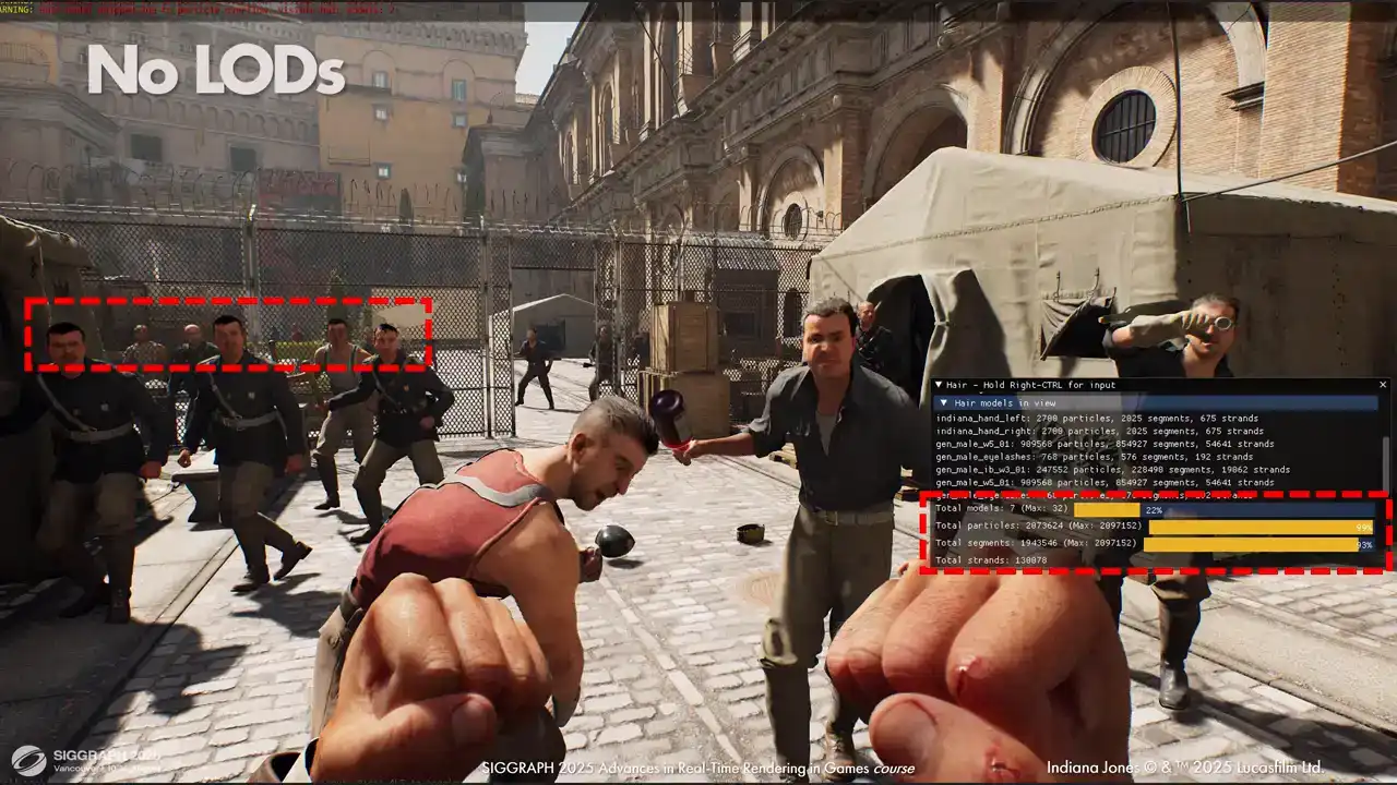
sterilization cost because that scales with the number of pixels covered and not with the number of segments themselves Here is a demonstration of how this helps us maintain a large number of characters with strength hair on screen Without Elodie we can only fit 7 hair models in a frame and two of them are actually in these hands. Other characters in the back don't get anything, as you can see, which is an issue in a game where you can walk into a crowded enemy camp. But with LODs we can fit everyone and maintain a good visual quality, and we still render the same number of segments.

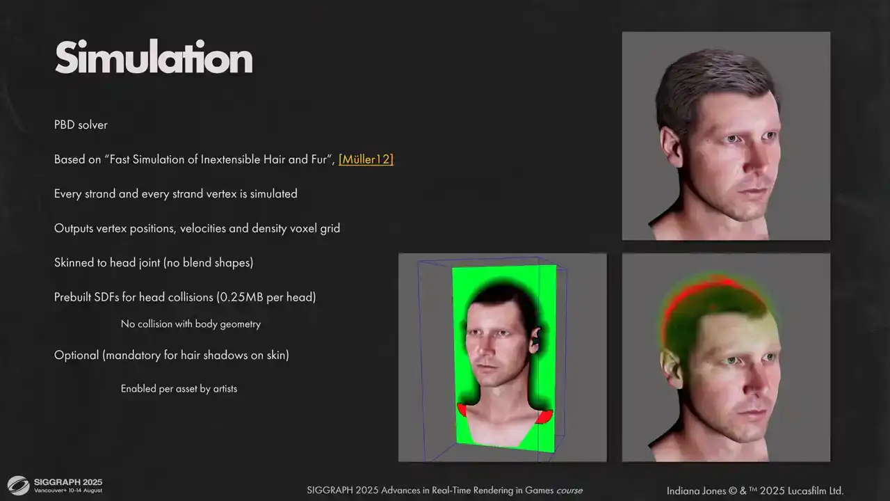
For simulation, we based our solution on Müller's work, Fast Simulation of Inextensible Hair and Fur. We simulate all strands and all particles in each strand. It happens before head skinning is applied, so we only account for main head joint movement at the time of simulation. For collisions with the head, we pre-bake head geometry into SDF. We don't do anything for head-to-body collisions because higher hairstyles in our game are not that long. When simulation step is over, we output local positions for hair vertices and their velocities for following passes. We also output voxel density grids for each simulation. We need that for hair collision and for hair shadow calculations. Next step is to find final positions for each hair vertex. Here we skin all hair strands directly to triangles on the base mesh. On asset import stage, for each strand root we compute the closest triangle on the parent mesh, its barycentrics and tangent frame. We store 80 bytes of information per strand root. Index of parent triangle, packed barycentrics, triangle normal and tangent. For TBN we use octahedral encoding. Head meshes have multiple LODs with different triangle indices, so we need to bake this information for each LOD of parent mesh separately. At runtime we always pre-skin all head meshes so we can just fetch transformed triangles from skinning buffers and transform hair strands accordingly. skinning is done, we transform hair vertices to clip space and store results for future calculations. It requires quite a significant amount of VRAM, but since we can reuse this data in multiple passes, it is well worth it. Later, on composition stage, we need positions per pixel to calculate motion vectors and interpolation coefficients for shading, so it is critical for us to cache transformed vertices.

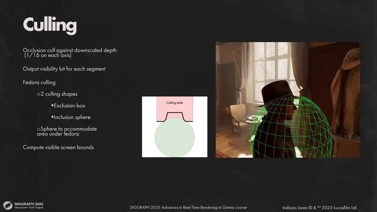
Now that we have our transformed vertices, we need to emit a list of segments to rasterize. We do a coarse culling stage here to discard invisible segments. We do three types of culling. Frostm culling, occlusion culling and head culling. For occlusion culling each segment is tested against downscaled depth buffer. If you have close up shots where each segment takes a significant portion of the screen, you might want to build a full high Z chain. But in our case just using 16 times downscaled depth buffer was enough. Last step is so called fedora culling. That is an iconic part of Indiana Jones and we have a lot of scenes where he puts the hat on and off, so we needed a solution to prevent hair clipping through the hat. We tried different approaches, but what worked for us was having two shapes. First is the exclusion box. It culls any segment above the hat. But as you can see, there is a small area right under the hat, where we don't want to cull any hair. To prevent it, we have a sphere that we cut out of the culling box to preserve these segments. If segment passed culling, we atomically raise the visibility bit for the segment. To reduce number of atomic operations, we utilize wave intrinsics and only do actual atomic write once per wave. Also during that stage, we compute real screen boundaries for each hair model to calculate how much space it needs in the visibility atlas. Let's move to rasterization. As you might know, hardware rasterization has some optimal performance when primitives you are trying to render are small. hair segments are definitely small, often much thinner than a pixel. There were other reasons for using software rasterization as well. We wanted to be able to offload as much work to a sync compute as possible, and it is easier to render perfectly anti-aliased lines like that as well. All those reasons combined moved us to writing our own software conservative rasterizer, optimized for short line segments. We consider each line segment a trapezoid and rasterize them into visibility buffer. Each shader lane gets one segment and rasterizes it using simple two-dimensional loops similar to what's shown on the slide. On each pixel we calculate its coverage, do a depth test against full precision, full rest depth buffer, and output it to visibility buffer using atomic operations. The algorithm is very simple but also very slow. It has a lot of dependent reads, cache utilization is far from ideal, and lane divergence is high. And not to mention that writing to multi visibility buffer is a slow operation by itself So how can we make it faster Let start by looking at our visibility buffer since writing to it is our most expensive operation by far We have three layers of fragments in each pixel, ordered by depth, and a separate layer with additive pixel coverage. To write the pixel to visibility buffer we use a simple code similar to what shown on the slide. This means our visibility buffer needs to be quite beefy, with 364 bit values per pixel and 32 bits for additive coverage. That resulted in 56 megabytes for 1080p just for the visibility buffer, which is a lot and we don't really want that. Using 64-bit Atomics is okay performance-wise, but to enable later optimizations and reduce memory footprint, we want to use 32 bits for our payload. Another issue is that this code has a lot of dependent atomic operations. It is quite slow. To fit the payload into 32 bits we need to compromise. We don't want to render too many segments on screen anyway, so limiting the maximum number of segments in a model to 22 bits was acceptable for us. That leaves 10 bits for everything else. We can reconstruct everything from segment index, but depth has to be in the payload for atomic minimum operation to work. However, 10 bits is not nearly enough for scene depth. What we do instead is we re-normalize and and linearized depth values inside model bounds. That way 10 bits is enough. We have a couple of z-fighting artifacts here and there, but they are not very noticeable. Another important consequence, we don't have any space left for hair model index in the payload. So we can't have two models output fragments to the same visibility buffer area. So instead of single full screen visibility buffer, we use an atlas of small tiles. Each Each hair piece allocates tiles from the atlas based on its screen space boundaries. Overlapping hair pieces will allocate different tiles, so each tile contains only one hair model. It also allows us to decouple memories spent on hair atlas from resolution, but it also comes with its own set of issues. Our atlas has a finite size, and overlapping hair models might require more tiles than we have in the atlas. We detect when it happens before austerization and downscale each tile until all tiles features fit into our atlas. It also has a nice side effect. We always have an upper boundary for strization because the number of pixels in the hair atlas is fixed. To avoid visible pixelization on downscaling we stochastically sample our atlas on final composition. We use Poisson disk distribution for that.

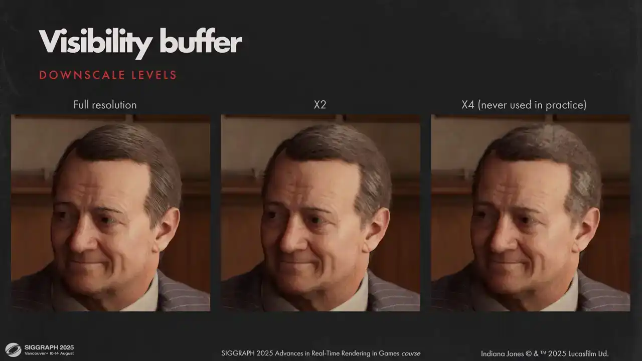
In theory we can fit almost unlimited amount of hair but in practice we never had to go further than half res. Here you can see how downscale looks visually. Usually it's active when you have multiple characters close to the camera and your display resolution is high enough. I mentioned earlier that we have three top layers in our visibility buffer, but usually a typical strand covers only about 20-25% of pixel area. Three front samples is not nearly enough to get opaque coverage. We didn't want to do order independent transparency because It's not very fast usually and complicates rendering considerably. We needed a fast approximation for combining dozens of fragments in a single pixel. What worked for us is to accumulate coverage additively using an anatomic operation and reconstruct alpha blended coverage later on composition stage.

To convert additive coverage to alpha blended, we make a few assumptions. First, we assume that all strands have similar screen space thickness. Second, we assume similar BSDF properties for all strands covering a single pixel. Given that, we can numerically simulate total coverage as a function of additive coverage by drawing a bunch of opaque lines and calculating precise total coverage after each line is drawn offline. Then, all we have to do is to approximate numerical data with a polynomial. We found that fifth-degree polynomial is a very good fit, but shipped with a quadratic approximation as it's slightly cheaper and gives more visually opaque results.

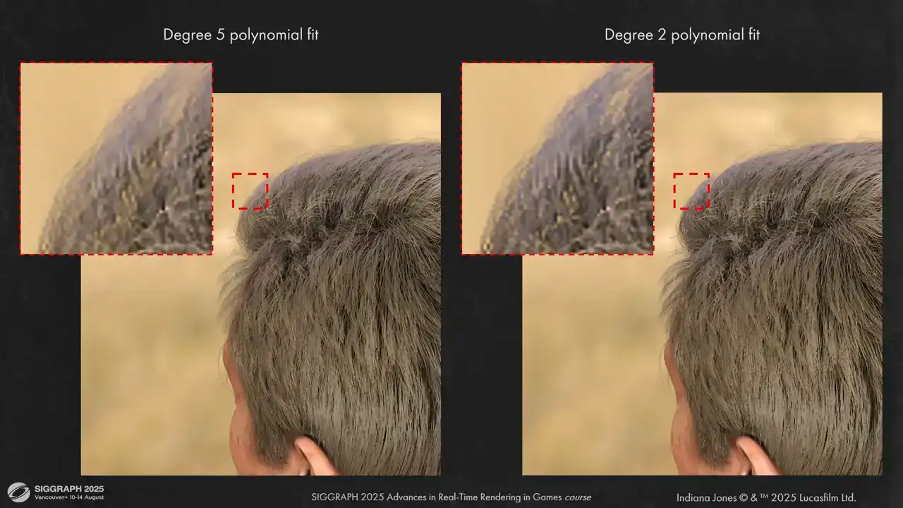
Here you can see the visual difference between two approximations. As you can see, visually results are very close to each other, but the second degree

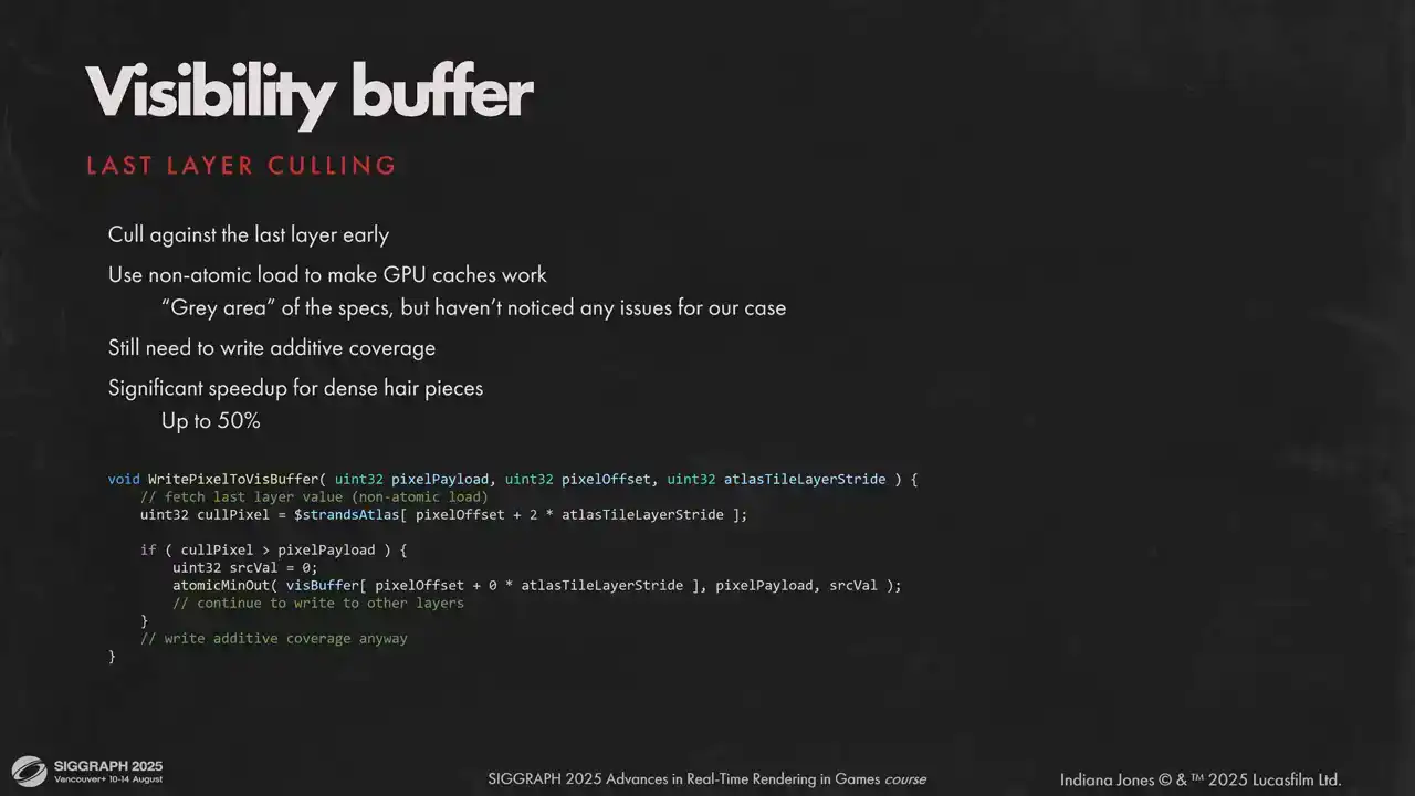
is a bit more opaque. One other sketchy but very efficient optimization we can cull early against the last layer of our visibility buffer. The catch is we can use non-atomic load to utilize caches. Atomic and non-atomic operations on a single memory location is a very grey area, but it saves quite a lot, up to half of the rasterization time for some models, and we didn't see any issues with the hardware that we shipped on.

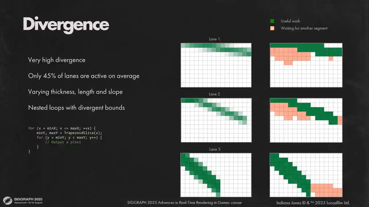
Let's move on. The other thing that we had to fight was very high lane diversions. On average, we had less than half of our lanes doing useful work at any given time. We had two nested loops with divergent bounds, and very different segments can end up in the same wave. Some might be thicker than the others, some might have different inclination, and because all instructions in a wave are executed in a lockstep, each lane must wait for its neighbors, even if this lane could have moved to the next column. You can see it illustrated on the slide. We rasterize each segment first top to bottom and then left to right. If any segment has active pixels in current column, all segments in a wave will wait for that segment. This is illustrated as orange dummy pixels. What we can do in that situation is we can flatten two loops into one and transform in a loop into a conditional statement that moves to the next column. So we rasterize different columns for different lanes at the same time. That way we can remove any diversions that come from different inclination and thickness. We will still diverge if the total number of rasterized pixels is different for segments

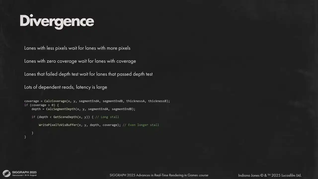
within a wave. Now that we removed one source of divergence, let's look at other sources. Lanes with less pixels still don't do anything at the end of rasterization loop. Also we have to do fine-grained depth test, and it's a source of divergence for fragments that pass the depth test and fragments that don't. Plus, all these operations are sequential and introduce stalls that are hard to hide. To deal with that, we defer expensive global memory operations. We allocate some LDS for pixel write requests and execute them in a bulk, once we have a full wave worth of requests. Lanes that don't have anything to do will skip the actual rasterization work on each iteration, but they will do global memory operations for other segments. we only did that for writes to layers visibility buffer but later added the same mechanisms for depth tests. You can add more stacks, but each stack adds some overhead to LDS, so I would only advise to use it for the most expensive divergent operations. Each wave in a workgroup gets its own stack space and these memory segments do not overlap. We need to store the payload for visibility buffer, which is 32 bits in our case, and also the pixel position and precise coverage. Because waves don't touch data of other waves, we don't need group LDS barriers, but we need wave LDS barriers. As you can see, we need quite a lot of LDS, so keeping your request payload small is key to get reasonable LDS usage and keep go-to occupancy. Here is an example of how pixel request stack works on an imaginary hardware with four lane waves. On the left you see the active lanes, on the right the state of the stack. On the first two iterations we don't have enough pixels on the stack, so we just add more requests. It's a fast operation and we are fine with diversions there. As soon as we accumulated enough data to fill a wave, we take top requests from the stack and write them to the visibility buffer. It's an expensive operation, but we have all lanes working on it. After that, we continue to accumulate samples, flashing them to the buffer and so on and so forth. Here are the results for our requests to lower lane divergence. We started with more than half of our lanes inactive on average. Flattening the loops reduced divergence by 10% and pixel request stack removed another 25%. And you can see clearly how it affected the timings. The shader runs almost two times faster. Now that our work is highly parallel, we face the next issue – low cache utilization. It happens because we randomize strands in the resource. Each lane tries to access different portion of the visibility atlas. Here you can see 4000 contiguous segments. They are all over the place. If we want good cache utilization, we need good spatial coherency for higher segments. The answer for us was global sorting for all segments in a model. We don't need it to be perfect, we just need segments in the same workgroup to be close to each other spatially. We divide the screen into buckets. Size of a bucket is close to the size of a Visibility Atlas tile, but it does not match it, because we can downscale Visibility Atlas, but we don't downscale the bucket size. In the culling path we populate bucket counters and do a simple counting sort. It is very fast, takes less than 100 ms. Here you can see the results. 4000 segments after sorting. But the granularity of the sorting is not perfect. We have found that doing another sorting inside each workgroup right before rasterization has a positive effect on performance as well although to a lesser extent We use large groups to rasterize hair and sort segments inside each work group according to Morton Curve This is a minor optimization it doesn save too much and depends on the hardware, so measure. We notice that different hardware performs better with different group sizes. Later we do strand space shading, and shading fetches a lot of per segment data. We can't use the same sorting order as we had for autorization. L2 cache hit rate will be low. So we need to sort the segments back to their original order. This time you don't need buckets, you can abuse the order in which GPU launches waves. Another way would be to store two lists, one for visible segments sorted spatially and another for visible vertices without any sorting. It would work just as well but then you will need more memory. That concludes the rasterization part. Let's move to shading. We shade strands per vertex to get smoother shading and safe performance. We use Marshmorm's shading model with approximation for reflection lobe from Brian Karras presentation at physically based shading course and other lobes from Sebastian Tafuri presentation at advances in real-time rendering. The model consists of three specular lobes. Untinted reflection, transmitted lobe visible when hair is backlit and the second tinted reflection lobe. We also added non-PBR scalars to each lobe, so for artist's convenience and some last-minute tweaks. I won't be diving too much into the shading model itself, there is a lot of good material on the topic. What we will focus on is self-shadowing. Marshaller model gives very

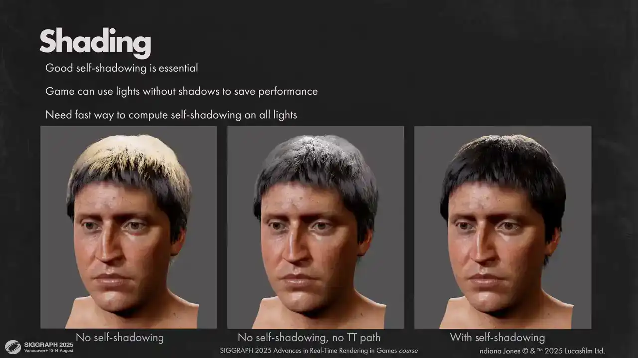
nice realistic results for human hair. However, both reflected and transmitted paths are very bright for most noncoming light directions. As a result, having good self-shadowing on all lights is absolutely critical for hair to look good. That places us in tough positions for two reasons. First, the game can use unshadowed lights that do not cast shadows to save performance. Second, is that even if we use only shadow casting lights, we have to keep the number of lights affecting the hair to a minimum. And setups for cinematics can be very complex. One easy trick we could do is to disable transmission path for unshadowed lights, but as you can see the results are still far from

ideal. Reflection path still has a lot of energy. For self-shadowing we considered multiple approaches. Deep opacity maps were considered at first but ultimately discarded due to memory requirements. Also having to rasterize each hair piece for each light was really a non-starter for us. Just rasterizing the hair into main view already takes significant portion of our budget. Second option that we thought of was to estimate global scattering at runtime by Raymarsh in hair density volume that we have from simulation passes. It is free on memory and it doesn't require extra australization passes. We can control the tracing speed by adjusting density volume resolution and number of ray marching steps, but it has scaling issues. Each hair shading point has to ray march a volume towards each light. But visual results that we get from that are generally good on most grooms. However, you can't get good high frequency shadowing with this approach. Also, some hair pieces require rather high resolution for density grid. For example, you can notice that this hair piece has quite visible self-occlusion artifacts. For our content, some grooms needed to have 256 voxels on each axis to resolve shadowing without artifacts, be that over-occlusion or leaking. Another option that we tried was a modification of the previous approach. Instead of ray marching towards the light, we do a fixed amount of ray traces stochastically to get a spherical visibility function for each shading point and encode it into spherical harmonic or spherical gaussian. Compared to previous option, we can adjust number of these visibility probes independently of shading points. We tried one probe per four vertices and the results were very similar to one probe per one vertex. Plus, we are no longer limited by the number of lights. We do one lookup to solve visibility, no matter how many lights affect the shading point. The downside is that it takes a lot of time and grid resolution has to be very high to avoid hair being too soft, similar to previous approach. For example, here is a visibility pass takes 6ms for a single hairpiece. We could have optimized it much further and throttle the workload over multiple frames, but visual quality will suffer and it's already not the

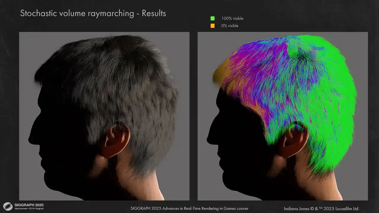
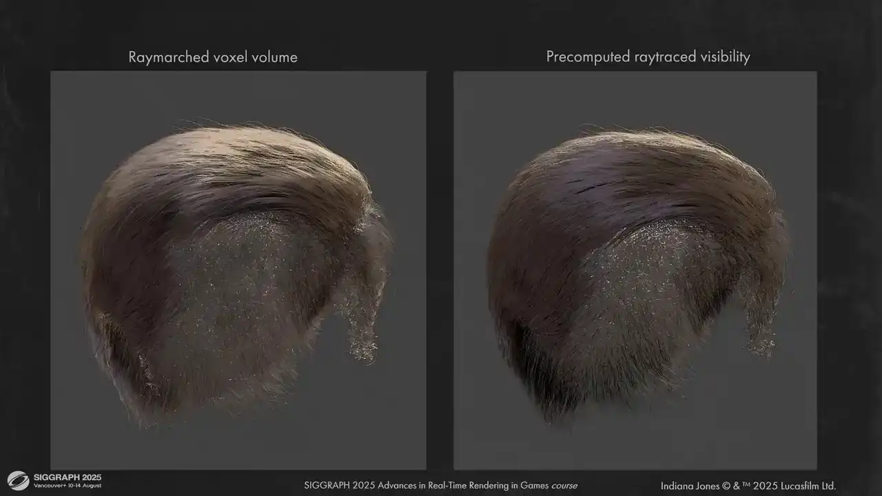
best. Here is how it looks on a simple groom. On the right you can see visibility representation for a single light. Lighting is plausible but a little bit flat.

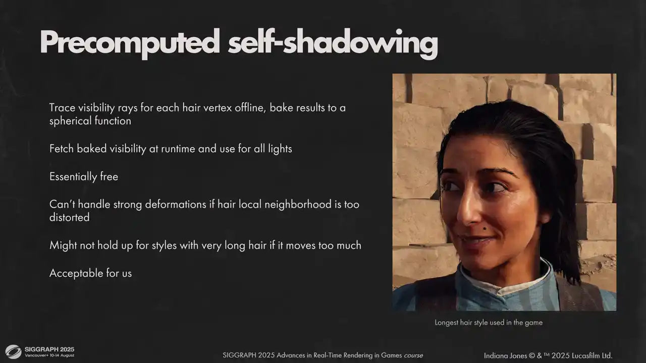
However doing that teached us a few things First is most of our grooms are rather static and short You can see the longest hairstyle we have on the slide And also for self shadowing what matters most is short neighborhood of each segment And it doesn't change too much under animation or wind With these constraints we could just bake our visibility one time and reuse for many frames Or what we actually shipped with do this baking offline with the software ray tracing instead of ray marching Using a ray tracer allowed us to have a good high frequency self-shadowing for each hair strands essentially for free, independent on the number of lights. We trace against the parent mesh as well, so hair is always shadowed by the head.

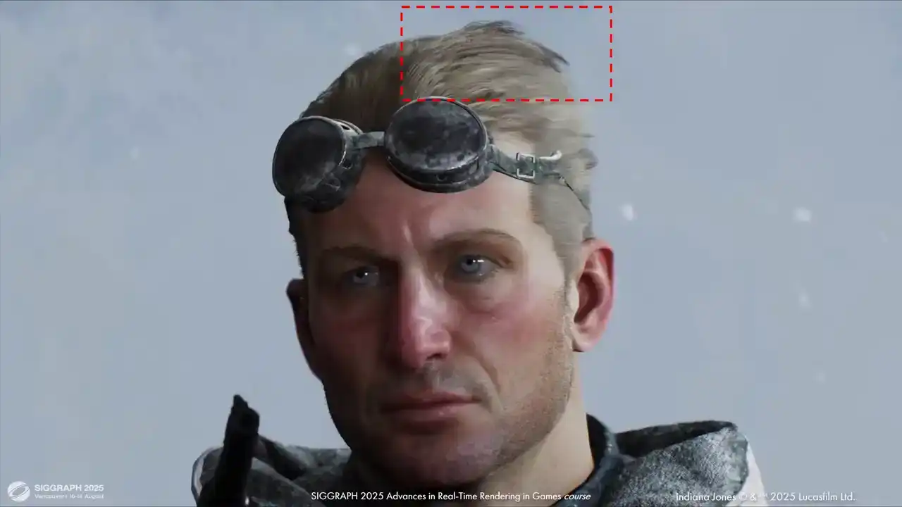
I was afraid that using baked visibility will break under motion, but honestly the results hold up quite well. You can see some artifacts under strong winds, like here for example, but it was acceptable

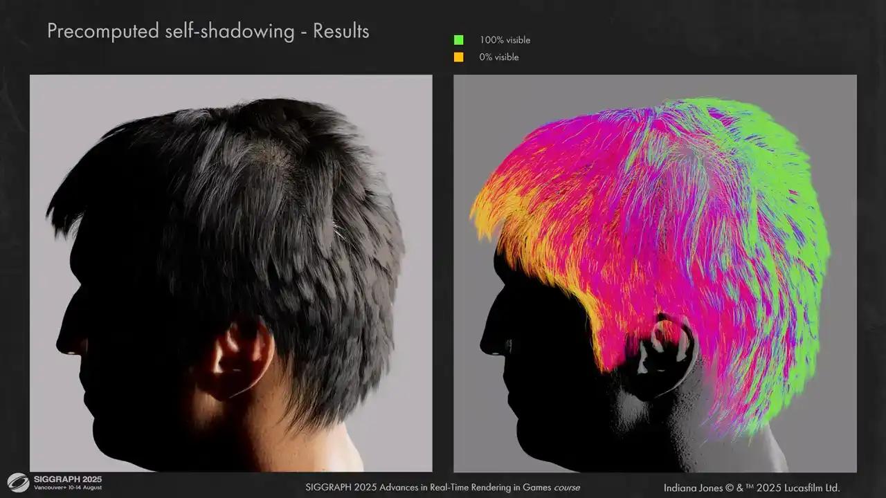
for us. Here are the results for baked ray traced visibility. You can see that it handles high frequency details very well.

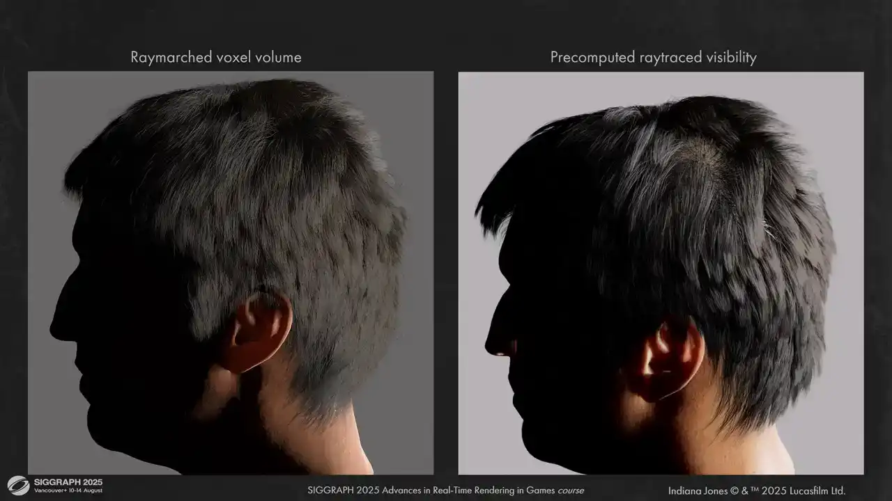
And here are some comparisons between volume ray marching and pre-computed ray tracing. The results are much less flat.

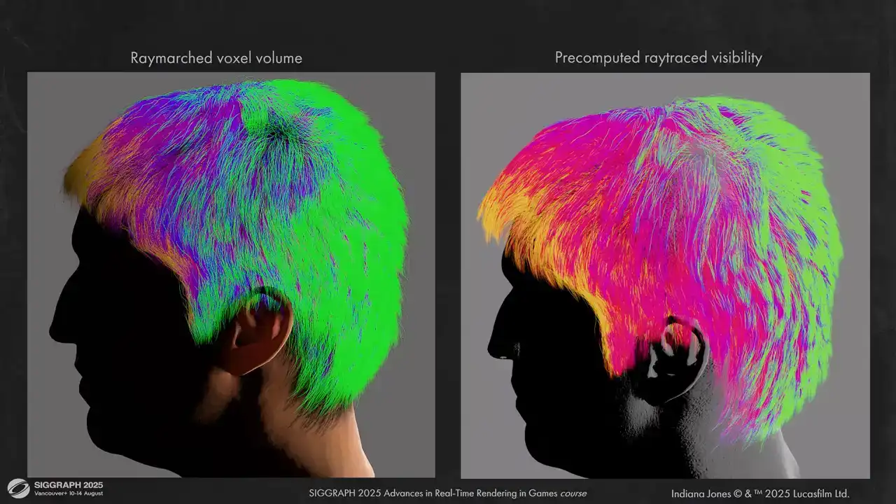
You can also see that the shadowing around the ear is more correct now. We don't have leaks like we have on the left.

And some other hair pieces. Here for example is Indiana Jones. You can see that self-occlusion is not a problem when we don't use voxel grids.

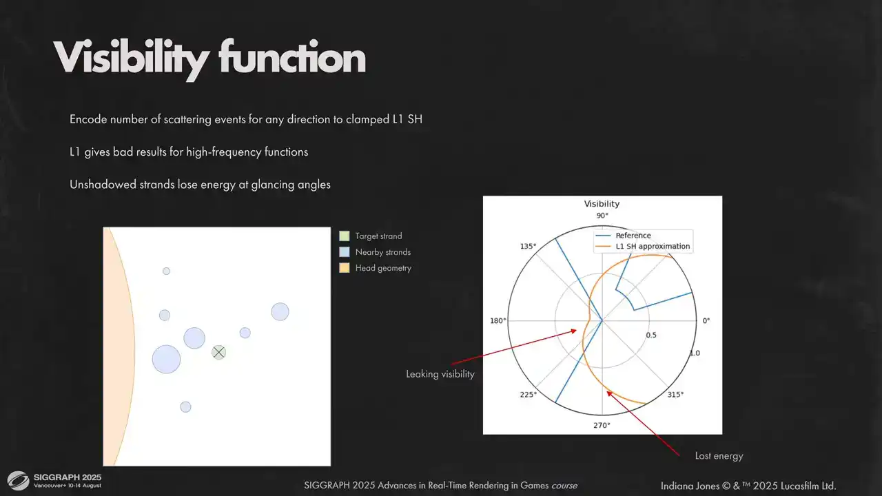
For visibility function we use clamped low-order spherical harmonic because of integration simplicity, low memory requirements and lack of ringing artifacts. Low-order spherical harmonics can't capture high-frequency data very well, so instead of encoding visibility directly, we encode the average number of scattering events in any given direction. Although when using spherical harmonics directly you can clearly see on the polar plot on the right that we lose high frequency angular details. It causes light leaking and energy loss.

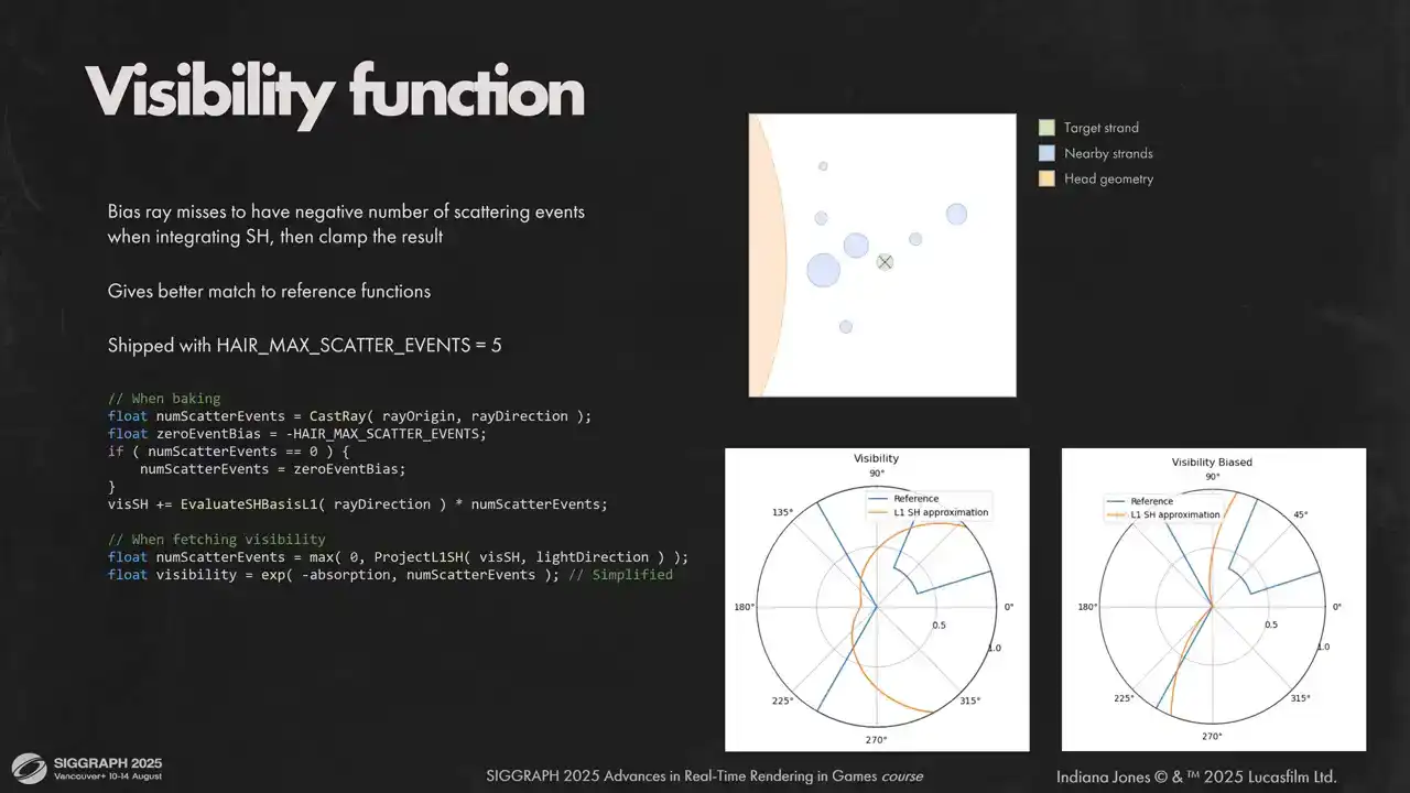
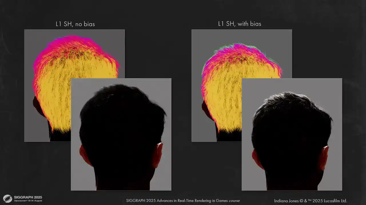
We combat this by biasing rays that did not hit anything. It helps us avoid overshadowing on glancing angles and get sharper transitions between light and shadow. Otherwise backlit hair will lose most of their glow.

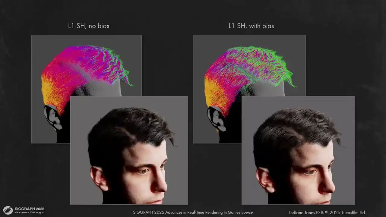
Here you can see how it looks on the actual content. Biases gives much more correct image and counter-backlit lighting is not lost.

For future work it would be interested to experiment with other spherical functions and dynamic recalculation for visibility, so we could handle strong winds and very long hair better.

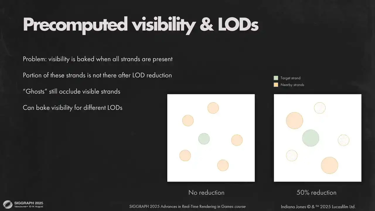
One other issue we have with pre-computed visibility is its interaction with our load system. We do loads by taking a portion of strands from the original model directly. That applies to pre-computed visibility as well. But this data was computed for unreduced model and contains collision with strands that were removed by the load system. Ideally, we would need to rebake visibility for every possible load, but it would take too much memory because we have as many loads as we have strands. That's why doing classic fixed-step LODs might have been a better

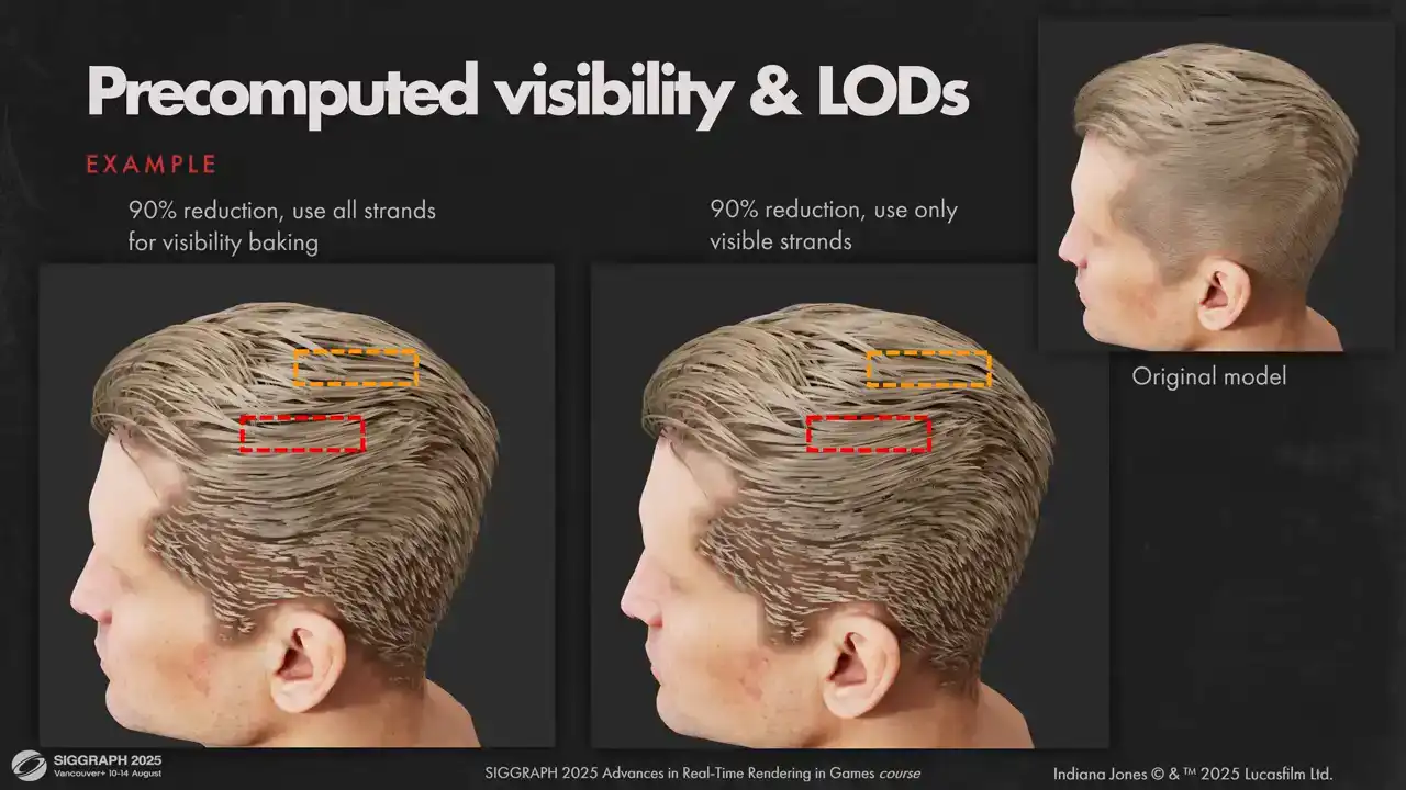
option. But in practice, the artifacts weren't too visible for us, so we kept the original lot system. You can see some very minor difference if you squint, but nothing too serious.

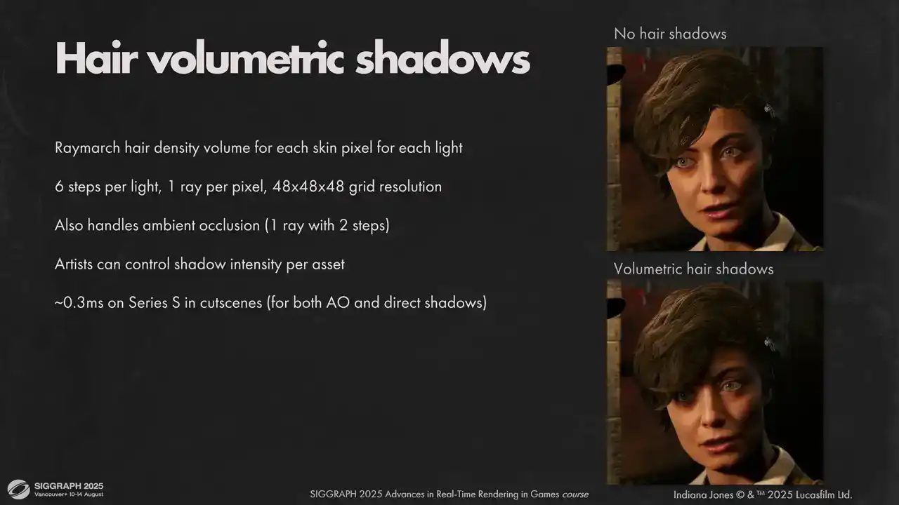
Note, now that self-shadowing is taken care of, we need to calculate shadows from hair on other objects. For skin pixel, we use volumetric raymar shadows, like one of the approaches we tried for hair self-shadowing. One extra bonus is that we can get ambient and specular occlusion with the same method. It is fast enough when you only do that for big pixels. It worked very well for hair, where shadow is usually naturally diffused. We don't need to rasterize strands into shadow maps, which saved some engineering efforts. Performance scaling is also acceptable. Unfortunately, the method is not perfect, our density volumes come from simulation, so it only supports skinny to one head joint, and thus it can't be used for fur on animals because, well, animals are usually pretty flexible. Also, we still need shadows from hair on other objects, and we didn't want to make some kind of acceleration structure for hair volume intersections. Usually missing hair shadow is not very noticeable, but it's not the case for the player character. You can see that missing shadow is very visible on the floor here, and we don't want to break the silhouette of our main character. For this case we did a very simple sculpted shadow proxy with inverted faces, that we

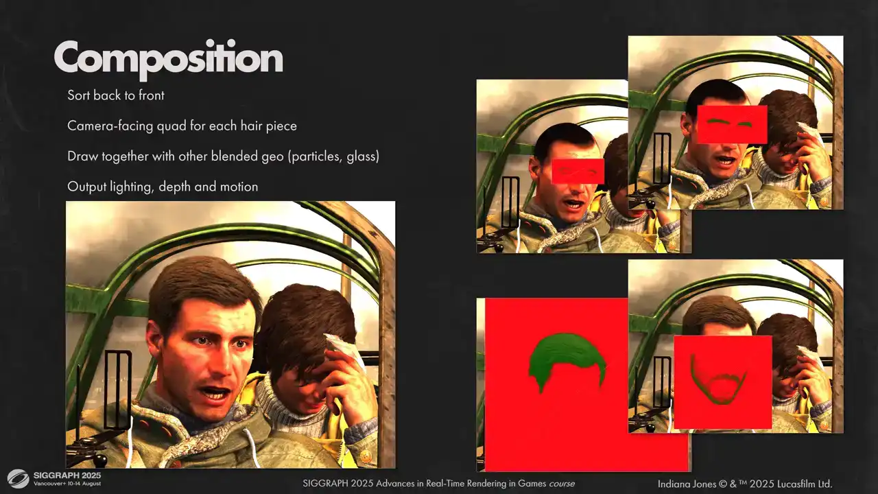
draw into shadow maps It is very fast to render and very simple for artists to make Now that we have our visibility and shading information for each hair vertex we need to compose it to final image Since each hair model has its own space in the visibility atlas, we must compose each model separately. We do that by drawing a camera-facing quad for each model. This is done together with other blended geometry in back-to-front order. It allows us to handle scenes with complex transparency setups in

in a unified way. Sometimes that might be a source of bugs. If the sorting is not correct, we have a few heuristics to help with that. We always try to draw a facial hair before main hairpiece. We bias all hair by half a meter when we sort objects. So smoke particles with soft blending are always drawn after hair when they are close together. We write hair to depth as we render it. so the particle soft blending works. It helps us to hide a couple of places where sorting has gone wrong, but we still have some less noticeable artifacts when sorting isn't correct.

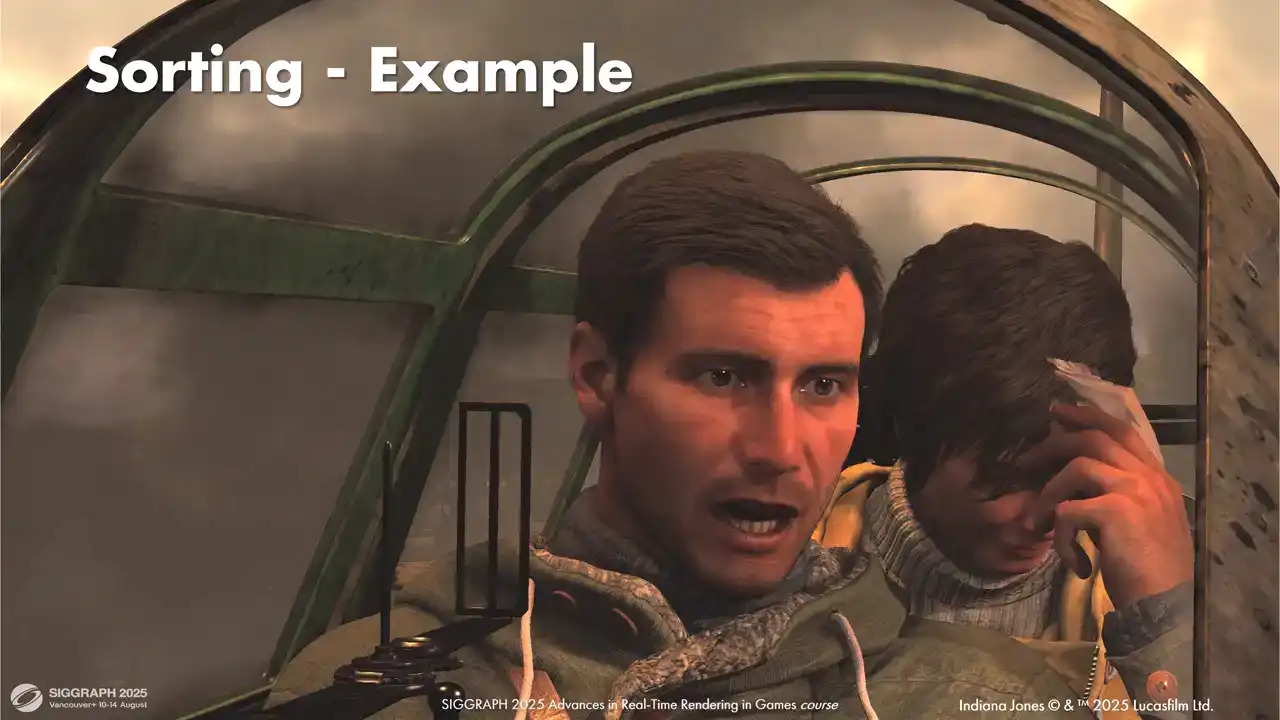
We didn't need to do a lot of manual tweaking, most setups worked out of the box. But some setups were complex and needed some fiddling with sorting biases. For example, take a look at this shot. Here we have a setup that was a bit problematic for us. Lots of overlapping transparencies and hair that is tricky to sort correctly. First, we render smoke behind the plane. Then is glass behind our characters. Gina's hair. Indie's eyelashes and eyebrows. Main hair pieces. And finally, the front glass in front of our characters. We had to tweak sorting biases on the glass and render front faces and back faces separately to draw everything in the correct order.

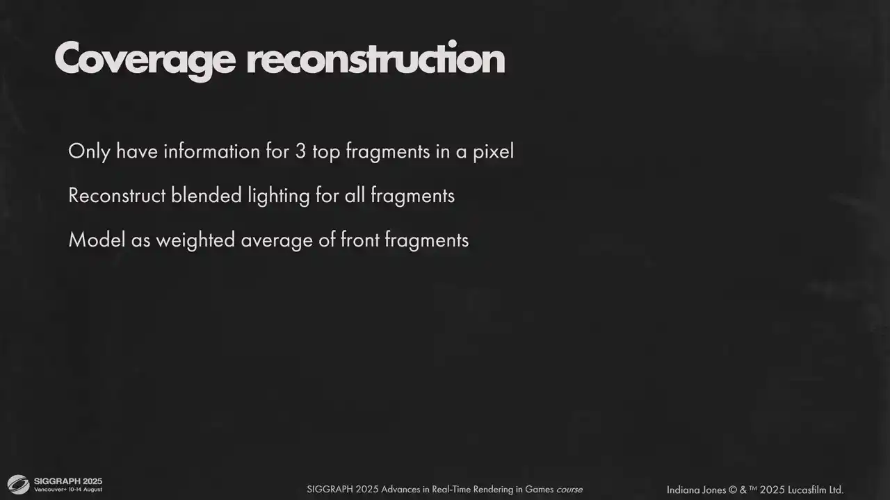
Let's look now at how we compose with one single hairpiece. As you might remember from the previous section, we only store three front segments and total coverage for each hair pixel. And we need to reconstruct the combined lighting for all hair fragments. We modelled the coverage from the first three samples as the regular alpha blended coverage. We also have our total coverage value from Visibility Atlas. We model the radians from missing part as a weighted sum of existing samples. We favour samples further away from the camera out of the three samples that we have, because they are closer to the samples that we want to reconstruct. This gives us a good appearance up close, where usually three front samples is enough, and at the distance, where more lighting information is reconstructed. Last but not least, motion vectors. Having good motion vector is crucial for upscalers, TAA and motion blur to work, so we wanted them to be perfect. Having a global post-transform vertex cache comes in handy here. What we do is we compress the cache we have and we use it in the next frame to calculate perfect motion vectors. Consoles and non-pass traced PC versions use first two components of post-transform hair vertex position, packed to two bytes each. It gives good results with a conservative raster that we use. However, if your authorization is not conservative and you rely on TAA to reconstruct the hair and you can afford an extra couple of megabytes, I would recommend using full precision for this. It considerably improves image clarity.

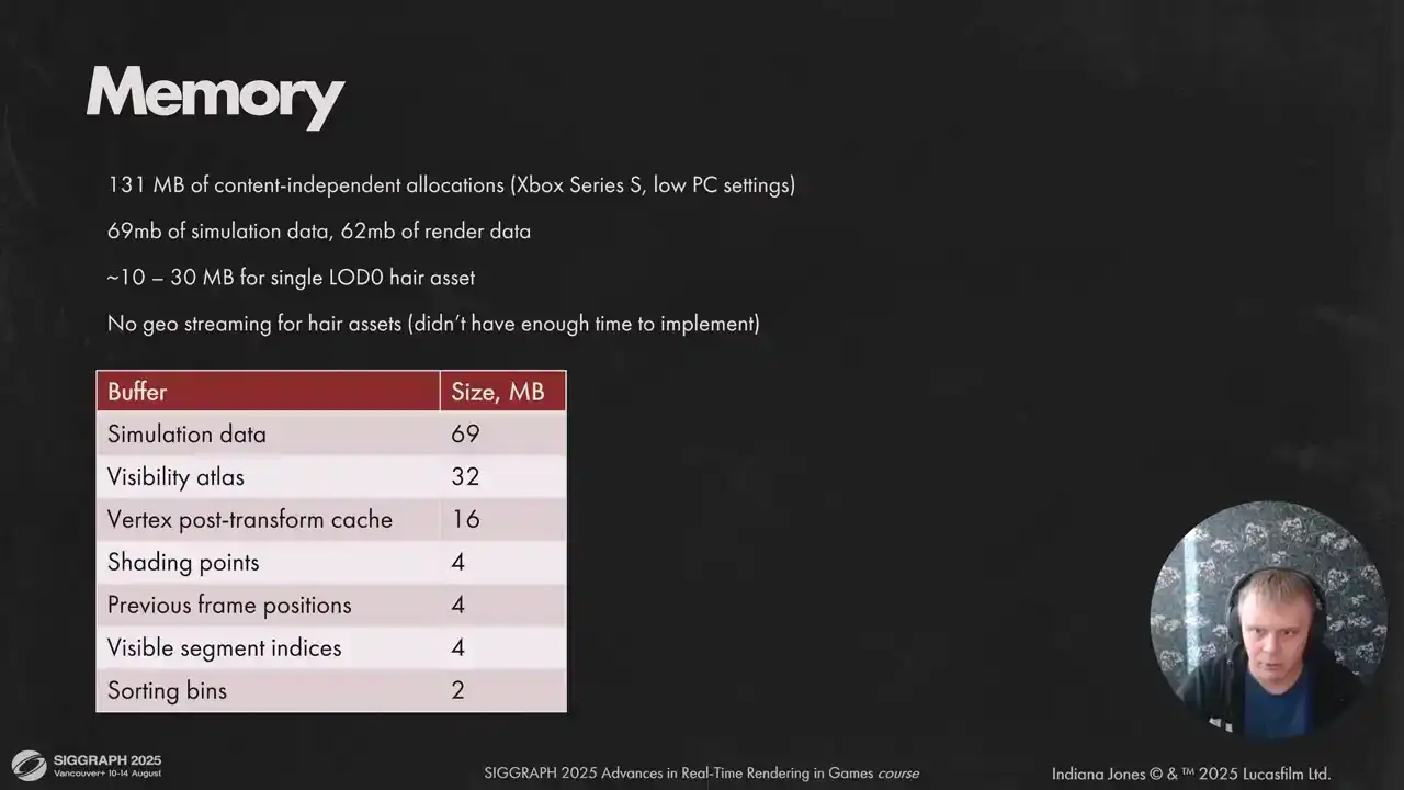
And here you can see how much memory we need for our low spec. For high spec we allow twice more strands, so it's 90 megabytes of render data instead of 62. We didn't have the time to implement hair streaming for assets, so resource-dependent memory load depends on the scene. For future work, we would like to reduce simulation requirements and implement asset streaming. On that note, I want to summarize what we have learned from our time developing StrandHair. The main point, in my opinion, is that StrandHair is fast enough now to be primary solution for hair on current gen hardware but you need to know your target and pick your battles accordingly also having a well-defined worst case scenario for all parts of the system helps tremendously because otherwise content will break all your limits eventually software rasterizer was also the right choice for strings it takes a considerable considerable amount of time to get it run fast but the result is well worth it. And lastly we need more work on the optimization front for dynamic hair. Right now we have to pick between performance and better hair movement. Thank you very much.